The skip list is my favorite data type. This may be because of some exposure to AVL trees back during my college days. Self balancing trees are wonderful, but they can be difficult to reason about.  If someone was to ask me what goes on when a value is inserted or deleted from an AVL tree, my answer would probably be “magic occurs”, and frankly, its magic I don’t care to dabble in.

Skip lists, on the other hand, are built on nice, classic linked lists. Linked lists get a bad rap when compared to List structures backed by an array, but they have their advantages. When comparing them to trees, it is important to realize that the trees are linked lists themselves.

The Basics

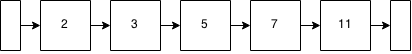
Figure 1: Ordered linked list

Skip lists are ordered lists – you traverse the nodes in order.  Much like this linked list is in order:

That’s well and good.  Inserting into it can be a bit of a pain though.  If you wanted to put a number in there… say 6, it would mean walking down the list one node at a time – is 2 > 6? nope… ok, 3 > 6? nope… ok, 5 > 6? nope… ok… 7 > 6? yes. So insert it before the 7.

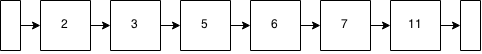
Figure 2: Ordered linked list after insertion

The number of checks that we do is proportional to the length of the lest and so this would be Big O of n – often written as O(n).

Lets look at what that list would look like as a binary tree instead?

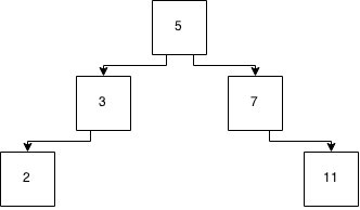
Figure 3: A tree

So now, to insert 6, we start at 5 (the root of the tree) and look to see if its greater than or less than 5.  As its greater than 5, we move down to the 7 node and check to see if its greater than or less than 7.  Its less than 7 and so we can insert this into the child spot on the less than side of the 7 node as that is empty.

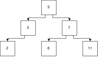
Figure 4: A tree after insertion

The tree took fewer steps to check (it took 2 checks for the tree vs 4 for the ordered linked list). The worst case for this is that it takes log₂(n) tests for a balanced tree. In Big O notation, this would be written as O(log 2). And this is better (faster) than the linked list.

The headache for the balanced tree comes when you now want to insert 8.

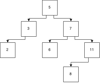
Figure 5: A tree after another insertion

But now, the tree isn’t balanced. And this means that in order to keep that log₂(n) performance for lookups, we need to rebalance the tree. There are several approaches to this. Red black, AVL, scapegoat, and splay are probably the best known of the self balancing binary trees. You’ll ultimately end up with:

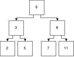
Figure 6: Tree after balancing

But note how many things moved round there to keep the tree balanced. This takes a fair bit of code to do and while it makes sense about how to do it, its not the easiest thing to get your head around.  Most of us just use TreeSet and let the standard library do it for you.

Lets go back to that linked list and make it kind of look like a tree of sorts to see if we can get the same benefits of being able to skip around in the structure with fewer comparisons.

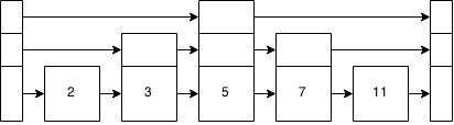
Figure 7: A linked list plus some added data

Just as with the tree from figure 3, you can see the layers and the tree structure imposed on the linked list.

Inserting a 6 is just, inserting a 6 into the linked list, very much like before. Except, now you start at the top of the stack and check there. That brings us to 5. Is 5 > 6? Nope. Top of the stack brings us to the end, so move down the stack and to the right. 7 > 6? yes? Move down the base level and insert the 6 between the 5 and the 7.

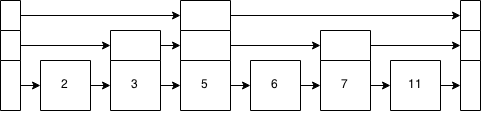
Figure 8: Linked list plus data after inserting a 6

Inserting an 8 is very much the same. 5 > 8? nope. Move down the stack and to the right. 7 > 8? Nope? Move down the stack because that level points to the end and we get to the base level. 11 > 8? Yes. Insert the 8 between the 7 and the 11.

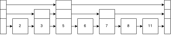
Figure 9: Linked list plus data after inserting an 8

As this is not a tree, we’re not going to get bent out of shape that it’s not balanced. However, in order to maintain the performance that approximates that of a balanced binary tree, we need to try to keep the stacks on top looking something kind of resembling a tree, even if it’s not perfect.

To do that, each time we insert a new node, we roll a dice to get how many stacks high it is. There are a few different methods for determining the exact nature of the dice roll.  One is using the maximum in the existing list (in this case 3). Another is to use the maximum for the allocation as the number to roll – typically this is based on other calculations of how big the list is or expected to be.  Another is to fix the dice to be no more than one greater than the existing maximum – so the next insert could be at 1, 2, 3, or 4 levels tall. Unless you are trying to get into the purity of the algorithm to do analysis on it – it doesn’t matter too much.

So, lets insert a 10 into the skip list. This was also done for inserting the 6 or 8, but was glossed over.  This is going to be very much the same as inserting the 8 before, just one spot more.

So, how high should the newly inserted node be? For this, we flip a coin – if its heads, we add another level. If its tails, we stop.  So, Heads, Heads, Tails. Two levels of additional pointers. Now the skip list looks like:

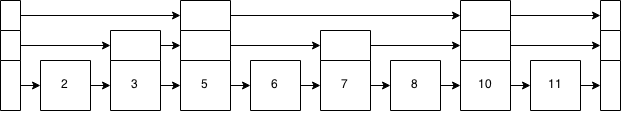
Figure 10: Inserting a 10

I was lucky with that coin flip in not having to redraw the data structure. But it can go as high as it grows. It is important that it is a coin flip to provide a gaussian distribution of node heights. That distribution is what gives you the log₂ performance that we associate with a binary tree. If it was some other function, that performance would be diminished.

Now, if we were to insert a 12, we can skip from the start to 5 to 10. Thus the name of the structure – a skip list.

The advantage here is that we don’t need to worry about rebalancing the tree. The probabilistic nature of the inserting levels will handle that for us.